


- Description
- L'opéra de Sydney et ses coques blanches au bord de l'eau, sous un ciel bleu.
- Source
- Bernard Spragg · original page
- Licence
- CC0 Public domain
 The Planning Fallacy
We know projects slip, and we plan ours as if it would be the exception.
In brief
- What : we underestimate timelines, costs, and risks in our own projects.
- Why : we reason from the most plausible scenario of this project, never from the distribution of similar projects.
- Detect : a single date, no buffer, “this time is different.”
- Avoid : outside view, ranges, measuring your past gaps, pre-mortem.
Definition#
 Illustration inspired by the person
 Fictitious illustration
The planning fallacy (planning fallacy) is the tendency to underestimate the time, cost, and risks of a future action, even when we know that similar actions took longer than expected. The term was proposed by Daniel Kahneman and Amos Tversky in 1979.
Two features distinguish it from a simple calculation error:
- it is one-sided: we are almost always wrong in the same direction (too short, too low);
- it persists despite experience: we know our past delays and plan the next one the same way.
The mechanism#
Kahneman and Lovallo distinguish two ways of forecasting:
Inside view#
We build a scenario: tasks, their sequence, available people. We infer the duration from it. Unexpected events are not included, by definition: you cannot plan what you do not imagine.
Outside view#
We look for the class of similar projects, check how long they actually took, and place the project in that distribution. Unexpected events are already included, without needing to guess them.
The inside view is natural; the outside view requires effort. Other drivers add to it:
- desire: the project must be accepted, so the optimistic plan wins;
- cause amnesia: we explain past delays by exceptional circumstances, therefore non-repeatable;
- the ideal scenario: we estimate effective working time, without meetings, interruptions, decision wait times, or fixes.
In a study by Buehler, Griffin, and Ross (1994), students had to predict the time needed to finish their honors project. Their average “realistic” estimate was about 34 days; the average actual duration was about 56 days, and only about 30% finished within the time they had predicted. Even their “worst-case” estimate was met by only a little under half of them. (Orders of magnitude reported by the study; verify in the source.)
Where you encounter it#
In project delivery#
- Initial sizing : pre-sales estimating, done with little information and a strong desire to succeed.
- Release planning and sprint commitments : capacity is counted as if no one were sick, interrupted, or blocked.
- Migrations and integrations : the areas where we discover the most surprises are the ones where we leave the least buffer.
- “Side” tasks : testing, documentation, deployment, training, data migration, underestimated or forgotten.
In management#
- Promises to the client or sponsor : a date stated in a meeting becomes a commitment.
- Last-minute requests : “it is just a small change”; the same error, repeated with every scope addition.
- Transformation plans : duration of change management, adoption, and skill ramp-up.
Estimating a semantic model or a loading pipeline based only on the nominal case overlooks reruns, acceptance testing variances in figures, and sources that change format. Estimate separately the happy path and the reconciliation cost, and compare with your previous projects rather than your intuition.
Famous cases#
Large-scale projects are the involuntary laboratory of the planning fallacy: their estimates are public, and so are their overruns. Bent Flyvbjerg, who studies major projects, made the Sydney Opera House a textbook case.
The Sydney Opera House 1957-1973#
Biases at play: planning fallacy, optimism, commitment before the project is defined.
What happened. In 1957, Danish architect Jørn Utzon won the architecture competition with a design of monumental shells on the harbor front. Construction began in March 1959, with completion announced for January 1963 and an estimate of 7 million Australian dollars. But the shell design had not yet been solved: the podium was built while teams were still figuring out how to build the roof, and the geometric solution did not arrive until 1961. Costs soared, the dispute with the new state government over payments and changes worsened, and Utzon resigned in February 1966, never seeing the project completed. The opera house was inaugurated on October 20, 1973 by Queen Elizabeth II; it cost 102 million Australian dollars, partly financed by a public lottery.

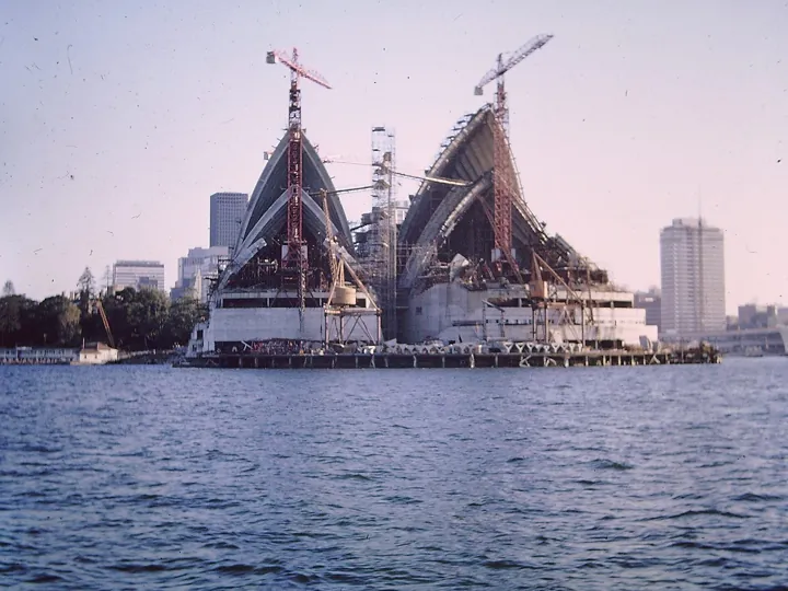
- Description
- The Sydney Opera House under construction, mid-1960s
- Source
- family photo published by its author · original page
- Licence
- CC0 Public domain
Sydney Opera House: planned, actual, and gap
Loading the chart…
View the data
| Planned | Actual | Gap | |
|---|---|---|---|
| Construction duration | 100.0 | 350.0 | 250.0 |
| Cost | 100.0 | 1457.142857142857 | 1357.142857142857 |
What this illustrates
The 1957 estimate concerned a project still at the sketch stage: this is the purest inside view. It assumed that what they did not yet know how to do would be resolved without extra cost. Two reflexes would have helped: compare with similar works (the reference class) and do not commit everything before the design is stabilized, by breaking the decision into stages.
Berlin Brandenburg Airport 2006-2020#
Biases at play: planning fallacy, illusion of control, minimization of technical risks.
What happened. Construction of Berlin’s new airport began in 2006, with opening set for October 2011. Delays piled up: in 2012, the opening was canceled just four weeks before the date, due to defects in the fire protection and smoke extraction system. Over the years, this was compounded by the bankruptcy of the planning company, that of Air Berlin, management changes several times, suspicions of corruption, and costly technical deficiencies. The airport finally opened on October 31, 2020, in a scaled-down ceremony, nearly nine years late and at a cost close to seven billion euros, versus about two billion announced.


- Description
- The tarmac of Berlin Brandenburg Airport
- Source
- NutzerAusBerlin · original page
- Licence
- CC0 Public domain
Berlin Brandenburg Airport: planned, actual, and gap
Loading the chart…
View the data
| Planned | Actual | Gap | |
|---|---|---|---|
| Construction duration (years) | 5 | 14 | 9 |
| Cost (billions of euros) | 2 | 7 | 5 |
What this illustrates
A single unresolved technical point (fire safety) was enough to shift the entire schedule: the plan assumed that every subsystem would be ready at the right time. Here, pre-mortem and intermediate validation milestones (testing critical systems early, not at the end of construction) would have exposed the risk in time. The parallel with an IT project is direct: final integration concentrates surprises.
Flamanville EPR: 54 months planned, more than twelve years late (France) 2006-2024#
Bias at play: planning fallacy (the start: a schedule based on an inside view).
What happened. On May 6, 2006, EDF’s board of directors decided to build an EPR reactor in Flamanville: estimated cost between 3,200 and 3,300 million euros (2005 value), 54 months of construction, and industrial commissioning announced for June 2012. First concrete was poured in December 2007. The schedule was then postponed many times: end-2012 grid connection announced in 2008, then 2014, 2016, fuel loading at end-2018, then end-2022 in the October 2019 forecasts. The reactor was connected to the grid on December 21, 2024. According to the Court of Auditors (2025), the total construction cost, including capitalized interest during construction, is about 23.7 billion euros (2023 value).
Where the bias appears. Jean-Martin Folz’s report (2019) judged the 54-month duration “totally disconnected from EDF’s latest experience”: 142 months from first concrete to fuel loading for Chooz B1, 98 months for Civaux 2, 100 months for Paluel 1 up to commissioning. The Court of Auditors (2020) similarly compares with the global average of 121 months. Setting the duration from an extrapolation of the N4 reactor, without confronting it with these references, is the hallmark of the planning fallacy, which consists of planning from the inside rather than from comparable cases. But both reports rank other causes first (project governance, studies not advanced enough, loss of skills), and the commercial context (a 48-month offer for the Finnish Areva/Siemens reactor) may also have encouraged displaying a short timeline: no document establishes whether the schedule was believed or chosen. Level of evidence: accepted, not proven. The gap with the references is established; its cognitive origin is an interpretation.
What this illustrates
Before approving a schedule, compare it to the duration distribution of comparable projects, including your own, and require each favorable gap to be explained by a specific reason. A duration announced as twice as short as all references calls for written justification, not agreement in principle.
Detection signals#
- “It should fit in two weeks.”
- “This time it’s different: we’ve done this kind of thing before.”
- The schedule contains only one date, with no range and no buffer.
- The estimate matches pure working time: no line for vacations, reviews, defects, or waits.
- The date was set before the estimate, and then the estimate was adjusted to it.
- No one can say how many past projects we are comparing against, nor what the gap was.
Avoidance reflexes#
- Take the outside view. Before estimating, list already completed similar projects or work packages, with planned and actual duration. The actual/planned ratio is the best information you have. (Flyvbjerg calls this method reference class forecasting.)
- Estimate as a range. Give three values: optimistic, likely, pessimistic. Commit to a high percentile (for example “4 times out of 5”), not to the best case.
- Measure your own gaps. Record every estimate and actual duration, then calculate the median and 80th percentile of the ratio. Use those numbers—not your intuition—to correct the next one.
- Break down, but add what breakdown forgets. Task-based estimation is useful, as long as you explicitly include integration, testing, reviews, deployment, and rework.
- Run a pre-mortem. “It’s six months from now, the project is seriously late: what caused it?” The exercise frees up people who see risks but do not dare mention them.
- Separate estimating from negotiation. The estimate describes the work; with a constrained date, what you can do is reduce scope, not compress the estimate. (See Anchoring.)
A calculation example (illustrative numbers)#
A team has completed twenty work packages of this type. The actual duration / estimated duration ratio has a median of 1.4 and an 80th percentile of 1.9. The new work package is estimated at 10 weeks.
| Commitment | Calculation | Announced duration |
|---|---|---|
| Without correction | 10 × 1 | 10 weeks (you go over in more than 9 cases out of 10) |
| One chance in two | 10 × 1.4 | 14 weeks |
| Four chances in five | 10 × 1.9 | 19 weeks |
Share of completed work packages by multiple of the estimate
Loading the chart…
View the data
| Completed work packages (%) | |
|---|---|
| ×1.0 | 5 |
| ×1.2 | 15 |
| ×1.4 | 50 |
| ×1.6 | 60 |
| ×1.8 | 70 |
| ×2.0 | 80 |
| ×2.2 | 85 |
| ×2.4 | 90 |
| ×2.6 | 95 |
| ×3.0 | 100 |
These numbers are made up for the example; what matters is the principle: the correction comes from the team’s history, not from a universal percentage.
With AI: detect, fix, mitigate#
AI is useful here because the main countermeasures (outside view, checklists, pre-mortem) require tedious, methodical work, which it does well and quickly. It does not replace your track record or knowledge of the context, and it will readily approve an optimistic plan if you present it that way.
Detect#
- Review an estimate or schedule and list what's missing: integration tasks, testing, acceptance testing, data migration, deployment, training, vacations, reviews, bug fixes.
- Spot optimistic language in status reports (“should,” “normally,” “just”).
- Compare an estimate against your exported history (tickets, milestones) and calculate the usual gap.
Fix#
- Turn a single estimate into a justified three-point range.
- Calculate from history the “one chance in two” and “four chances in five” durations.
- Propose a complete breakdown from a checklist of often-forgotten tasks.
Mitigate#
- Run an automatic pre-mortem at every milestone.
- Play the devil's advocate: a skeptical developer who challenges every assumption.
- Integrate estimate review into the ticket template or planning ritual.
Prompts to integrate into your workflow#
1. Critical review of an estimate. Use before communicating an estimate.
You are an experienced, skeptical project manager. I am going to give you a project estimate.
Do not approve it out of politeness: your role is to find what's missing.
1. List likely forgotten tasks (integration, tests, acceptance testing, data migration, deployment, documentation, training, vacations and absences, reviews, bug fixes).
2. List implicit assumptions and undated dependencies.
3. Say whether the estimate describes an ideal scenario or a realistic scenario, and why.
4. Propose a range (optimistic / likely / pessimistic), specifying what you are basing it on, and flag what you cannot know.

Estimate: [paste estimate here]
Context: [team, technologies, constraints]
2. Calibration against your history. Requires a tool that can run code; otherwise, verify the calculations.
Here is the export of our last [N] batches (columns: identifier, type, initial estimate in days, actual duration in days).
By type, calculate the actual duration / estimate ratio: median and 80th percentile. Do the calculations with code and show them.
Then apply these ratios to the new estimate of [X] days and give the “one chance in two” and “four chances in five” durations.
Flag if the sample is too small or too heterogeneous to draw conclusions.
3. Pre-mortem. Run at kickoff, then at each milestone.
We are six months in the future. The project described below is [six weeks] late and the client is unhappy.
Write ten plausible causes of this delay, from most to least likely, based on what is stated in the description (no generalities).
For each one: one observable early signal, and one preventive action to decide now.

Project: [description, team, schedule]
4. Blind estimation. Use before giving your own number, so as not to anchor it.
Estimate the effort for this work in days, with a range, based only on the description. I am deliberately not giving you my estimate.
Detail your reasoning by component and indicate the points where your estimate is most uncertain.

Description: [scope, constraints]
How to integrate them#
- In the process: prompt 1 is part of the checklist for every estimate; prompt 3 is part of kickoff and every milestone.
- In tools: keep these prompts in the wiki or in ticket templates, with a “estimated vs. actual gap” field to fill in at the end of each batch, which will feed prompt 2.
- In the ritual: during planning, one person reads aloud the points raised by AI, as you would read out risks in a review.
Precautions#
- Language models are themselves sensitive to anchors and sycophancy: they tend to go along with the user (Sharma et al., 2023). Present the work to be critiqued without signaling that you are attached to it, or explicitly ask for a contrary view.
- A range produced by AI is plausible, not measured: without your history, it remains just another hypothesis.
- Do not paste confidential data (clients, contracts, people) into a tool not authorized by your organization.
Limits#
- The outside view assumes past projects are comparable; otherwise it misleads in the opposite direction.
- Not all delays come from estimation: moving scope, dependencies, and team departures also weigh in. The bias explains part of the slippage, not all of it.
- A systematic buffer can be “consumed” by work that stretches out (Parkinson's law): the buffer is useful only with tracking.
Sources and verification#
- Kahneman & Tversky (1979), “Intuitive prediction: biases and corrective procedures,” TIMS Studies in Management Science, 12 — origin of the term.
- Buehler, Griffin & Ross (1994), “Exploring the "planning fallacy",” Journal of Personality and Social Psychology — the study on undergraduate theses.
- Lovallo & Kahneman (2003), “Delusions of Success,” Harvard Business Review — inside view and outside view.
- Flyvbjerg (2006), “From Nobel Prize to Project Management: Getting Risks Right,” Project Management Journal — reference class forecasting.
- Klein (2007), “Performing a Project Premortem,” Harvard Business Review.
- Sharma et al. (2023), “Towards Understanding Sycophancy in Language Models” — language model sycophancy.
- Guinness World Records, “Largest proportional increase in cost for a building project” — the Sydney Opera House (7 → 102 million Australian dollars, construction from March 1959 to 1973).
- Airport Technology, “Berlin Brandenburg opens, ending a decade-long debacle” — timeline and costs of Berlin Brandenburg Airport.
- Jean-Martin Folz (October 2019), “La construction de l'EPR de Flamanville,” report to the Chairman and CEO of EDF — establishes the 2006 forecasts (54 months, June 2012), successive announcements, and the gap with EDF's construction durations.
- Cour des comptes (2020), “La filière EPR,” thematic public report, summary (English version) — compares the planned 54 months with the global average of 121 months and describes the underestimation as blatant.
- AFP via Connaissance des énergies (January 14, 2025), summary of the Cour des comptes report “La filière EPR : une dynamique nouvelle, des risques persistants” — reports grid connection on December 21, 2024, twelve years after the planned date.
See also#
Combines with, or reinforces#
These biases feed each other.
Related biases#
Variants or cousins: not to be confused.
- Hofstadter’s Law
- Loi de Parkinson (concept or method, no page)
